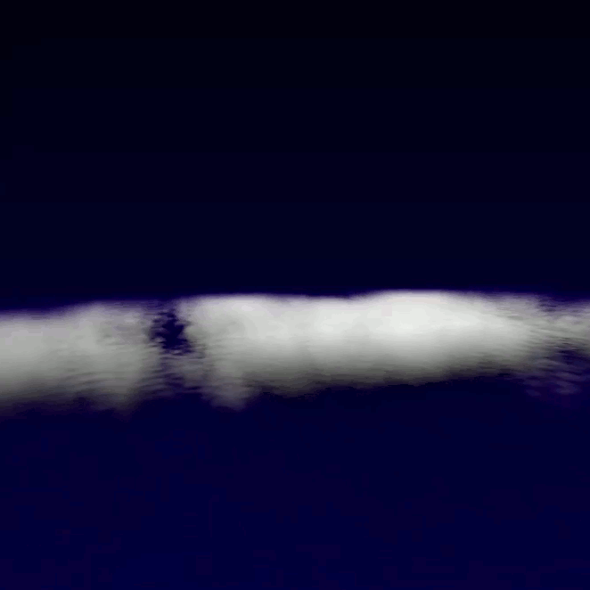
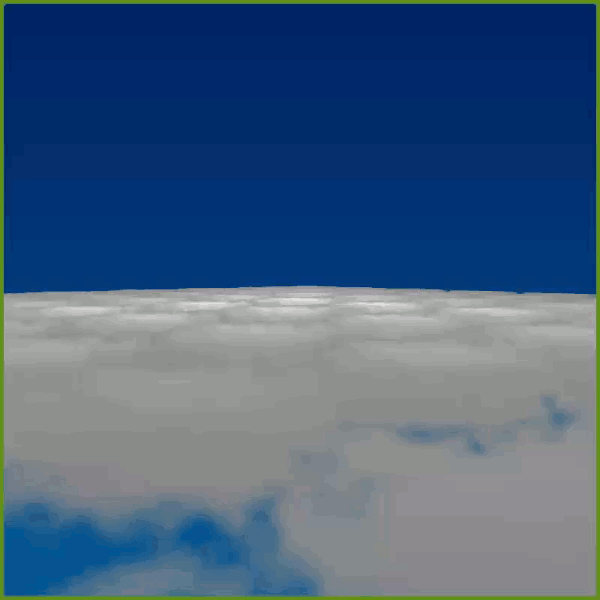
Finally we wanted to add some simple textures and play around with different settings such as camera position. For the background we decided to go with a simple gradient generated inside the shader prior to rendering the clouds:
A real cloud consists of many-many water particles spread out at random. Each particle is tiny and spread out at random with (typically) a lot of empty space between particles. A real light ray is scattered all over the cloud in variety of directions. It would incredibly difficult and computationally intensive to replicate reality-based ray tracing algorithm.
Our simplified approach was to shoot a ray towards the light source from our original ray as it passes through the cloud and sample densities from that point towards the light source. Then we continue marching though our clouds repeating the process. This is done for every ray shot through our cloud.
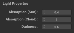
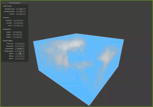
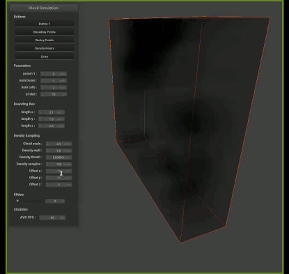
The most difficult part of ray marching the cloud is correctly mixing the “marched densities” with color for final output. In order to pick the correct mixing parameters, we added three additional setting to our GUI. This enabled us to play with ray marching settings on the fly.
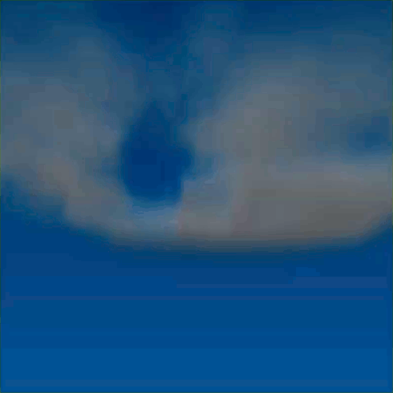
After a lot of tinkering with values and textures, we were finally able to get realistic looking clouds that resemble our goal (left image). Lastly we added a gradient background to the rest of the scene (right image).
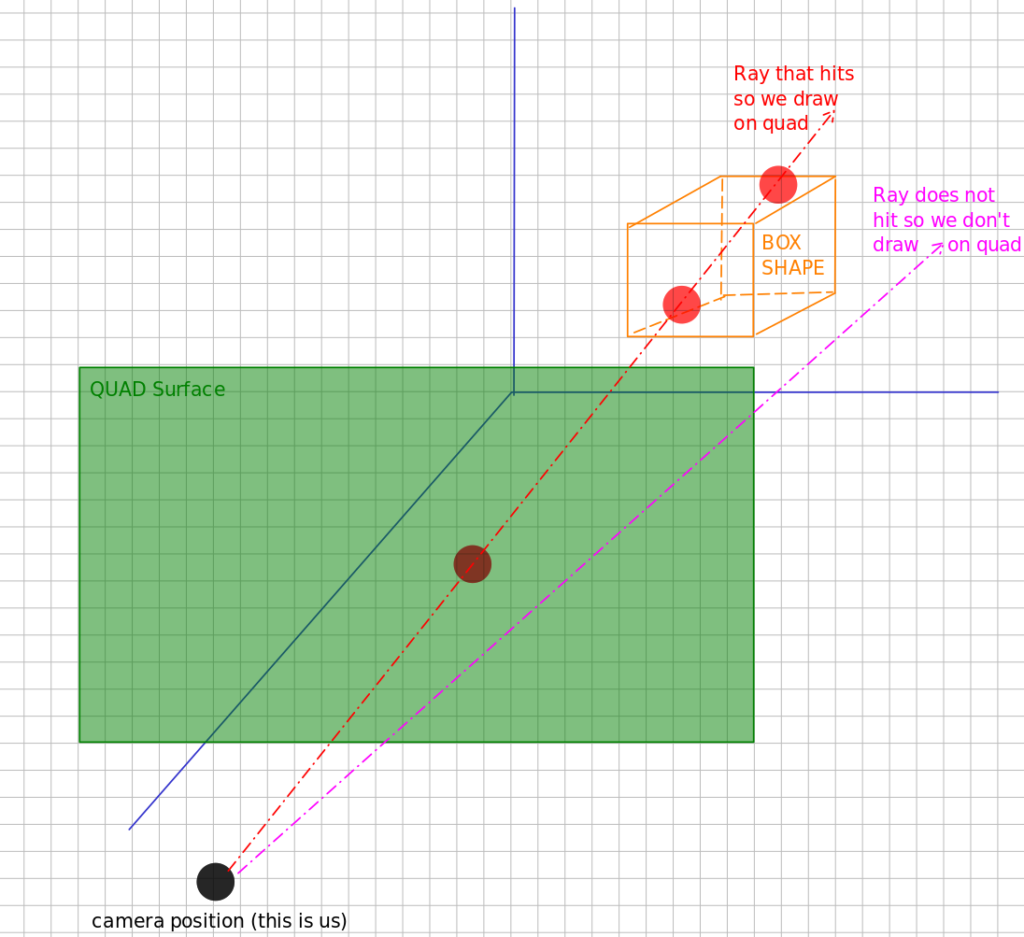
Next step was to “place our texture into the box”. The idea here is to shoot a ray from the camera towards the box. If the ray intersects the box, we will sample our texture at multiple points along the ray inside the box and then draw that point on the quad surface.
If the ray does not intersect the box, we do not draw our texture on the quad.
This enables us to have full control over where to place our clouds in the scene as we reshape and move around the bounding box.
Prior to ray tracing, we generated a bounding box structure using two 3-dimensional points.
The two points represent rear-leftmost-lower point & front-rightmost-upper corners of the bounding box. These points enabled us to shift x, y, and z coordinates to obtain the remaining 6 corners (total of 8).
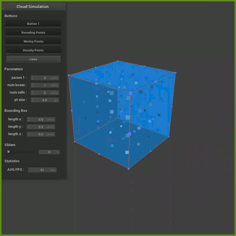
Given the 8 corners, we were able to generate 12 lines outlining our volume using GL_LINES primitive (please see thin orange outline). Then, from the same points, we generated 12 triangles representing our bounding volume planes (please see light blue & 50% transparent walls). These were done using GL_TRIANGLES primitive.
Lastly we have added three sliders to our GUI in order to manipulate the bounding box: length x, length y, and length z. These simple parameters allow us to easily resize the bounding box volume in three dimensions.
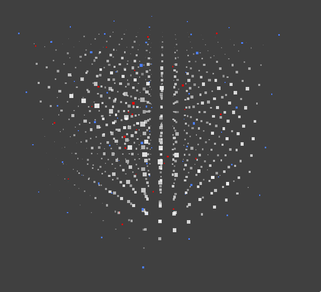
After testing our Worley Noise algorithm in 2D, we extended it to work in 3D space. The computational demand of our algorithm was really high because we had to calculate the min_distance(every_pixel, every_random_worley_point).
In order to minimize the computations, we split up the cube into sub-sections and placed one random point in each sub-section. Now, every pixel has to check it’s distance against random worley noise points located in 26 adjacent sub-sections in addition it’s own section (total of 27 checks per pixel).
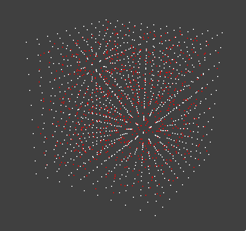
Red dots: Worley Noise White dots: Cell boundaries
Red Dots: Worley Noise White Dots: Density
Worley Noise
The biggest challenge was in blending cube edges as we replicated the Worley Noise. In short, for the sub-sections touching the outter-planes of the cube, we had to offset our worley noise points to the correct location in order to compute correct distances.
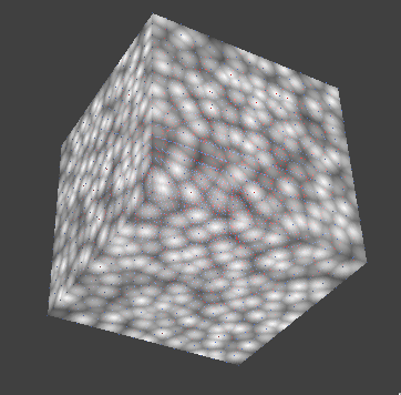
After some debugging, we were able to quickly replicate our Worley Noise texture successfully:
Compute Shader Limitation:
Initially we wanted to speed up the distance calculations by using a compute shader. Unfortunately after implementing a basic compute shader, part of our dev team was unable to run the project due to OpenGL 4.4 (required for compute shaders) incompatibility with Mac OS.
First task in generating realistic clouds was to pick pick an implementation approach. We settled on Worley Noise technique. The idea is to scatter random points all over the screen and find the distance between every pixel and it’s closest point. Then, we would use that distance to shade every pixel with a value between 0 and 255 scaled by the distance.
To test our 2D Worley Noise generation algorithm, we used a simple LodePNG library in order to generate .png files.
First we shaded the background in white color and randomly generated n points. At this stage there is an optimization worth mentioning: evenly subdivide the screen into rectangles and place only one random point per rectangle. This way, every pixel in the scene has to be checked only against a rectangle it belongs to in addition to neighboring rectangles.
Next we found a closest distance between each random point and every pixel in the scene. Normalized by max distance and multiplied by 255 – we now able to shade our scene. The figure displayed on your right is the inverted result [ 255 – normalized_distance ].