Abstract:
We combine tessellating Worley and smooth noise patterns with Beer’s Law and the Henyey-Greenstein phase function to model ray-tracing through cloud formations of varying densities, sample rates, and light properties.
Technical approach
Clouds have a characteristic shape in the popular imagination. We learned that one approach to generating the cloud is using a combination of 3D Worley noise and smooth noise. Combined in three dimensions – those noises result in cloud like appearance. Then we pass the texture to OpenGL shader for ray tracing and ray marching. In order to tackle this problem, we stripped down Project 4: Cloth Simulator code.
Generating Cloud Textures
The process starts with seeding a bounding box with numerous random points (known as Worley points), then calculating the closest distance to the nearest Worley point for every pixel. We use an optimization to reduce the computational demand – by dividing our bounding box into a grid of nine cells and only adding one Worley point to each cell, we can limit the number of “nearest point” calculations for each pixel to just 8 in 2D, and 26 in 3D. Having the distance from each pixel to the nearest Worley point provides the framework for generating the overlapping circular shape of a cloud’s edges, but in order to create seamless cloud textures that don’t abruptly end if the camera position changes, we “wrap” the Worley point formation. This is done by duplicating the bounding box (grid cells and Worley points included) until the original is surrounded (by 8 clones in 2D space, and 26 in 3D space), then using adjacent Worley points in the clones in the nearest point calculation.
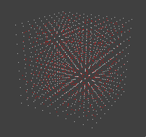
Red dots: Worley Noise
White dots: Cell boundaries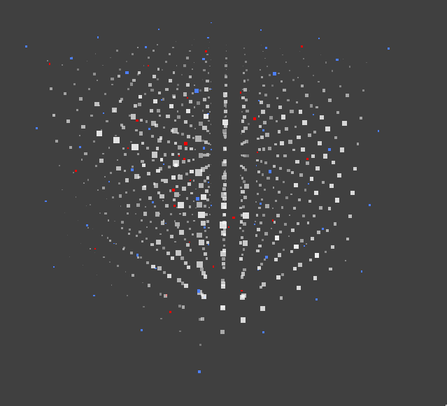
Red Dots: Worley Noise
White Dots: Density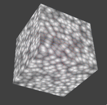
Worley Noise
Implementing Worley noise was mostly a matter of following the prior work of others, but we did add our own twist by decoupling a number of parameters, including the texture resolution and the size of the Worley point grid cells.
Worley noise provides decent outlines for our clouds, but is rather lacking when it comes to texture. To populate our Worley cloud scaffolds, we turned to Perlin noise, a type of gradient noise often used for textures. But in the end, we utilized smooth noise instead, because our Perlin noise implementation did not look right. In 2D, the smooth noise generation process involves trilinear filtering on every pixel. Extending the technique to 3D space was a design choice we made to make our clouds more realistic.
Then, we combine the Worley and smooth noise using the scale function described in Fredrik Haggstrom’s “Real-time rendering of volumetric clouds” thesis.
Raytracing
At this point, we have created a cloud texture that we then passed into our shader. Inside the shader, we placed our texture in a rectangular shape. At first we were misunderstanding how to render our texture and were outputting the texture on the surface of the rectangle:
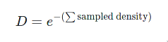
Eventually we figured out that a proper approach to this problem was to use a quad implementation. The idea is to shoot a ray from the camera at the quad intersecting our texture container. For each ray that intersects our texture, we will sample the texture with an adjustable sample_rate. Using the Beer’s law, we will calculate the output pixel onto the quad. This method enabled us to properly draw the clouds onto the scene and manipulate the cloud placement, cloud size, and our point of view.

Raymarching
Next step was to add light to our clouds. In order to do this, as we shoot a ray through our texture: for each sample point, we shoot another ray towards the light source, adding up the light landing at every texture point between the light source and our sample point. This gave us an overall light estimation for every sample point on our ray. Combining light for every sample point, we got the total light output for that pixel on the quad.

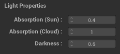
The Henyey-Greenstein equation was useful in adjusting the light angle falling on our cloud. Additionally, we placed a variety of scalar adjustments in our GUI for this part of the project in order to help with troubleshooting and dialing in our settings.

Technical Difficulties
We encountered a series of hiccups involving the MacOS operating system and OpenGL. Many of the OpenGL functions that would enable quicker texture generation via GPUs are only found in the latest versions of OpenGL, and we encountered compatibility issues on the MacOS operating system. This forced us to abandon compute shaders and make our texture generation run on the CPU instead. Using OpenMP helped parallelize parts of the process, but it is still computationally intensive and therefore our program takes few seconds to initially generate our textures.
Rendering to the BBOX was aesthetically displeasing, so we changed our implementation to render to Quad. At this point, our noise started to resemble real clouds flowing within the box.
The lack of typical debugging tools, like print statements, in the shader forced us to adapt to using color outputs as a proxy for understanding what our code was doing. This was a new coding paradigm for us and took some adjusting to.
Future Approaches
If we were to do it again, we would likely make the following changes:
First, we would probably use a platform agnostic technology like WebGL, one that would run on any operating system. This would have circumvented the compute shader compatibility issues we encountered, and make our project accessible to a wider audience.
Our GUI slows down substantially during computationally intensive rendering (when sample rate is increased beyond 60 samples); making the draw interpolation frame independent instead of using a fixed update rate would allow the GUI to be operable even when textures are rendering.
Contributions
- Zachary modified the cloth simulator project to create the scaffold for our cloud generation project, converted the noise algorithms to run in 3D space, figured out the bounding box and quad rendering, and implemented ray tracing.
- Roman was our webmaster, created a 2D noise prototypes, handled the 3D ray marching, debugged multiple parts of the code, and served as subject matter expert for all things lighting related.
- Callam was our wonderful video expert, handling everything from voiceovers to post production edits.
- William modified the GUI to improve the user experience, and handled the majority of the write-ups.
Results
We have achieved our goal to render volumetric clouds. Our GUI enables us to adjust the size and placement of our clouds. Additionally we are able to adjust variety of paremeters such as light location, sample rate, and scale among many others. Also, we can adjust our point of view.
Below the clouds with a star texture backdrop 
Above & through the clouds with gradient backdrop 
Above the clouds with dark gradient backdrop and bright light
You can view our GitHub repository here.
References
- Olajos, Rikard. (2016). Real-Time Rendering of Volumetric Clouds [Master’s thesis, Lund University]. ISSN 1650-2884 LU-CS-EX 2016-42. https://lup.lub.lu.se/luur/download?func=downloadFile&recordOId=8893256&fileOId=8893258
- Häggström, Fredrik. (2018). Real-time rendering of volumetric clouds [Master’s thesis, Umeå Universitet]. https://www.diva-portal.org/smash/get/diva2:1223894/FULLTEXT01.pdf
- Lague, S. [Sebastian Lague] (2019, October 7). Coding Adventure: Clouds [Video file]. YouTube. https://www.youtube.com/watch?v=4QOcCGI6xOU
- Vandevenne, L. (2004). Lode’s Computer Graphics Tutorial. Texture Generation using Random Noise. https://lodev.org/cgtutor/randomnoise.html